mdsa-tools

Tools for systems-level analysis of Molecular Dynamics (MD) simulations

Pipeline overview

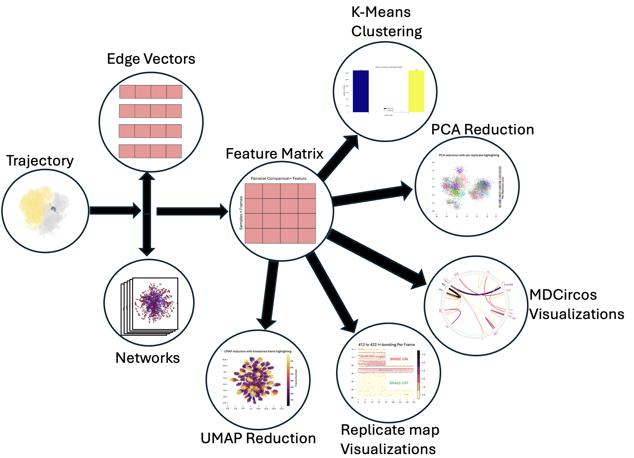
We start from an MD trajectory and generate per-frame interaction networks. We represent theese as edge vectors (vectors consisting of just the edgeweights for every edge connecting pairs of unique nodes); stacking these per-frame vectors yields a feature matrix suitable for clustering (e.g., k-means) and dimensionality reduction (PCA/UMAP). Results can be visualized with graphs, scatter plots, MDcircos plots (residue H-bonding), or replicate maps of frame-level measurements of interest.

Install

pip install mdsa-tools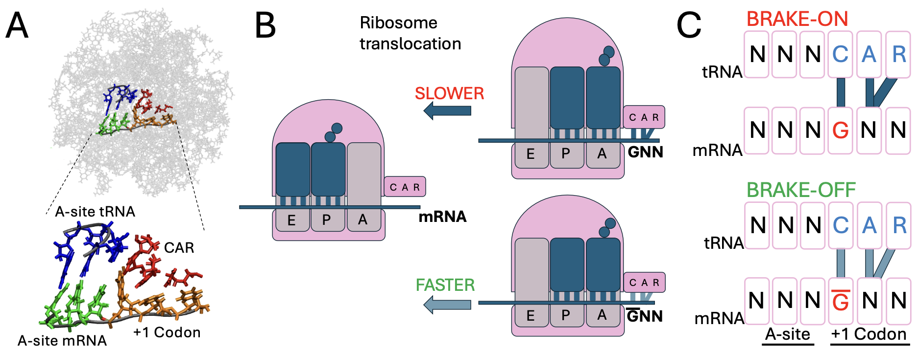

Systems Problem Area:

In the Weir Group at Wesleyan University, we perform molecular dynamics (MD) simulations of a ribosomal subsystem to study tuning of protein translation by the CAR interaction surface — a ribosomal interface identified by the lab that interacts with the +1 codon (poised to enter the ribosome A site). Our "computational genetics" research focuses on modifying adjacent codon identities at the A-site and the +1 positions to model how changes at these sites influence the behavior of the CAR surface and correlate with translation rate variations.

Development Note:

Moving forward the most recent work will be through github releases and PyPI pushes will be the most recent confirmed covered working release.

Quickstart example (see docs for more examples):

from mdsa_tools.Data_gen_hbond import TrajectoryProcessor as tp
import numpy as np
import os

###
### Datagen
###

# load in and test trajectory
system_one_topology = '../PDBs/5JUP_N2_CGU_nowat.prmtop'
system_one_trajectory = '../PDBs/CCU_CGU_10frames.mdcrd'

system_two_topology = '../PDBs/5JUP_N2_GCU_nowat.prmtop'
system_two_trajectory = '../PDBs/CCU_GCU_10frames.mdcrd'

test_trajectory_one = tp(trajectory_path=system_one_trajectory, topology_path=system_one_topology)
test_trajectory_two = tp(trajectory_path=system_two_trajectory, topology_path=system_two_topology)

# now that it's loaded, make objects
test_system_one_ = test_trajectory_one.create_system_representations()
test_system_two_ = test_trajectory_two.create_system_representations()

np.save('test_system_one', test_system_one_)
np.save('test_system_two', test_system_two_)

###
### Analysis
###

from mdsa_tools.Analysis import systems_analysis

all_systems = [test_system_one_, test_system_two_]
Systems_Analyzer = systems_analysis(all_systems)

# transform adjacency matrices, perform clustering and dimensional reduction
Systems_Analyzer.replicates_to_featurematrix()
optimal_k_silhouette_labels, optimal_k_elbow_labels, centers_silhouette, centers_elbow = Systems_Analyzer.perform_kmeans(outfile_path='./test_', max_clusters=5)
print('clustering successfully completed')
X_pca, weights, explained_variance_ratio_ = Systems_Analyzer.reduce_systems_representations(method='PCA')  # you could do method='PCA'/'UMAP' here
print('reduction successful')

###
### Visualization
###

import matplotlib.cm as cm
from mdsa_tools.Viz import visualize_reduction

# visualize embedding space with original clusters
visualize_reduction(X_pca, color_mappings=optimal_k_silhouette_labels, savepath='./PCA_', cmap=cm.plasma_r)

# map transitions between various cluster assignments
from mdsa_tools.Viz import replicatemap_from_labels

fake_labels = np.arange(0, 18, 1)
replicatemap_from_labels(cmap=cm.plasma_r, frame_list=[9] * 2, labels=fake_labels, savepath='./Repmap_')  # 9 frames each