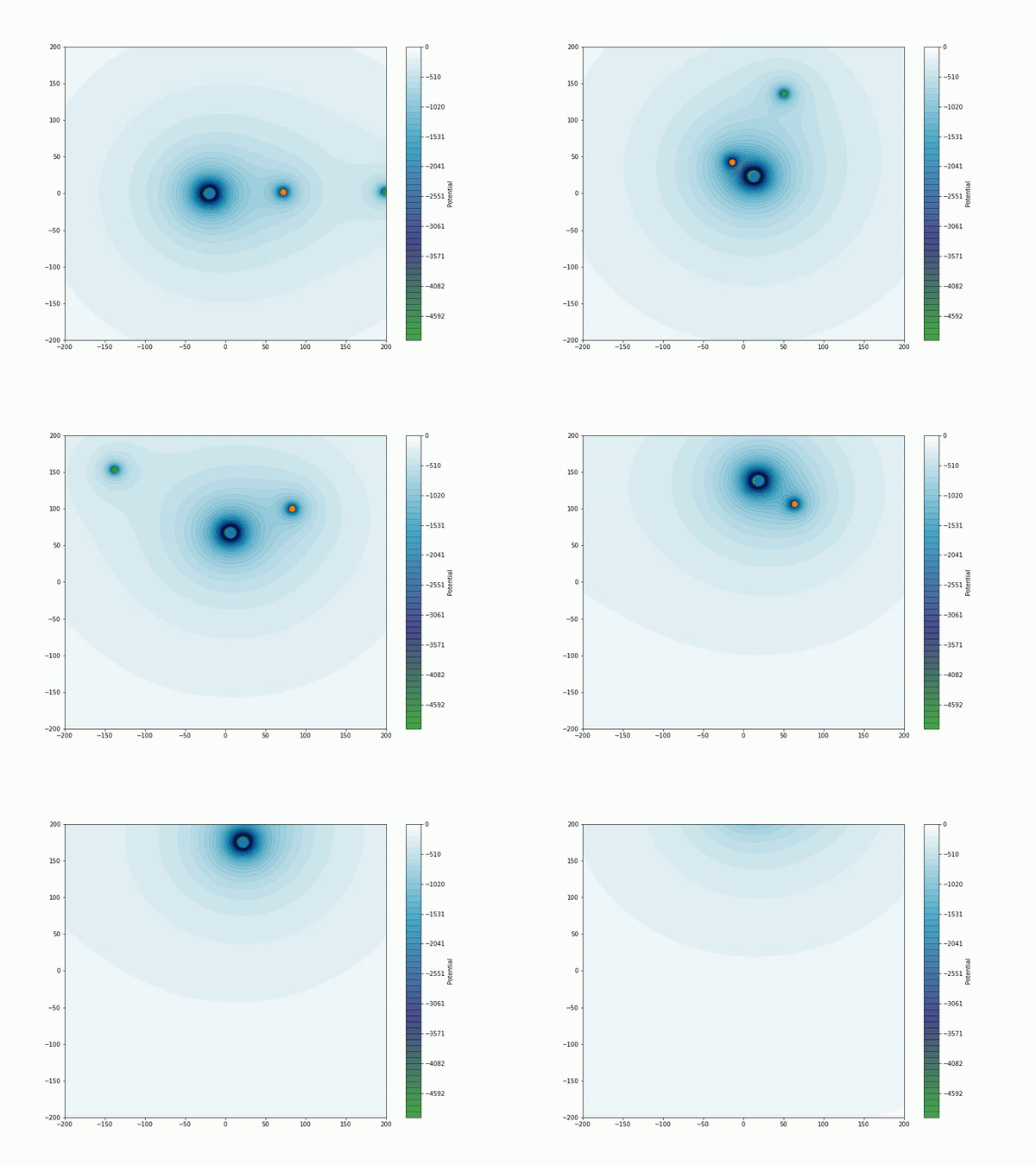
Welcome to the world of Barnes Hut Algorithm! This repository contains the code and documentation for the Barnes Hut Algorithm, a popular and powerful method for approximating the forces acting on a large number of particles in a three-dimensional space.
Barnes Hut Algorithm is a clever method for simulating the behavior of a large number of particles in a three-dimensional space. It's commonly used in computational physics and astrophysics to model the motion of celestial bodies such as stars and planets. The algorithm uses a quadtree or octree data structure to divide the space into smaller regions, and approximates the forces acting on each particle by considering the forces acting on groups of particles in nearby regions. This allows the algorithm to achieve high accuracy while significantly reducing the computational cost.
There are several advantages to using Barnes Hut Algorithm over other methods for simulating particle interactions:
- Efficiency: Barnes Hut Algorithm can simulate the behavior of a large number of particles in a much shorter amount of time than other methods, making it ideal for large-scale simulations.
- Accuracy: Despite its speed, Barnes Hut Algorithm can produce highly accurate results that are comparable to other, more computationally-intensive methods.
- Flexibility: The algorithm can be customized and modified to suit a wide range of applications in physics, astrophysics, and other fields.
In this implementation, the Barnes-Hut Algorithm is implemented using a quadtree data structure. The particles are inserted into the quadtree based on their position, and each node of the tree stores the total mass and center of mass of the particles in its sub-tree. This allows for an approximate calculation of the gravitational force acting on each particle, reducing the overall computational complexity of the simulation.
The barnes_hut.py file contains all the important classes and functions needed to simulate particles using the Barnes-Hut Algorithm. Users can import this file to create their own simulations.
Point class
The Point class creates a point in space with position and velocity vectors.
Rectangle class
The Rectangle class creates a boundary within which a quadtree can function. It is used to define the simulation space and the boundaries of each node in the quadtree.
Quadtree class
The Quadtree class creates a quadtree within the desired boundary. It is used to store particles and calculate the gravitational forces between them.
If you'd like to contribute to Barnes Hut Algorithm, we welcome your contributions! You can submit bug reports, feature requests, or pull requests through GitHub.
This code is released under the MIT License, which means you are free to use, modify, and distribute it as long as you include the original license in your distribution.
I'd like to thank the original creators of Barnes Hut Algorithm for developing such a powerful and useful method for simulating particle interactions. I'd also like to thank the open-source community for their contributions to this project, as well as the developers of the various libraries and tools used in this code. Last but not the least thanks to @iamstarstuff for supporting me through multiple blocks during the way.
Whats new: Barnes Hut Algorithm implementation to simulation.
Glance of the Update.
The project is focused on simulating the motion of bodies obeying inverse square law.
#Main function :
def step(mass:'arr', x0:'arr',y0:'arr',vx0:'arr',vy0: 'arr',dt=0.1, G = 1):

    x1 = x0 + vx0*dt
    y1 = y0 +vy0*dt

    vx1 = []
    vy1 = []
    #Loop over planets to find the distance:
    for i in range(len(x1)):
        x1self = x1[i]
        y1self = y1[i]
        ax = 0
        ay = 0
        for j in range(len(x0)):
            if i == j:
                continue
            x_dist = x1[j] - x1self
            y_dist = y1[j] - y1self
            Rsq = x_dist**2 + y_dist**2

            # Contribution from the jth mass:
            a = G*mass[j]/Rsq
            ax += a * x_dist/np.sqrt(Rsq)
            ay += a * y_dist/np.sqrt(Rsq)
        vx1.append(vx0[i] + ax*dt)
        vy1.append(vy0[i] + ay*dt)

    return x1,y1,np.array(vx1),np.array(vy1)
The step() function will take the "initial positions/previous positions" of the bodies as inputs and give their respective "present positions". This is done in the following way:
- The function
step()takes:
mass(masses of all the bodies in one array)x0(x position of all the bodies in one array)y0(y position of all the bodies in one array)vx0(x component of velocities for all the bodies, also in an array)vy0(y component of velocities for all the bodies, also in an array)dt(component of time)G(Gravitational Constant (for visualization purposes G=1)
- Find the latest x and y positions, denoted as x1, y1:
- This is done by using the kinematic equation:
$x = x_0 + v_{x_0}t$
$x_0 = $ initial x_position (=x0).$v_{x_0}$ = initial x component of velocity (=vx0)
Similarly for y1.
We proceed to make two empty lists for "Velocities" that we shall update within the loop.
- We make a loop to calculate the acceleration and update the velocities. This process loops over the number of bodies and finding their acceleration using
the Newton's Gravitation formula: $ F = ma = \frac{GMm}{R^2}$.
After this, we find the component of acceleration$a_x, a_y$ .
Then we append (add)$v_{x_1} = v_{x_0} + a_x*dt$ to thevx1 =[]list (similarly for vy1).
realistic.planets.mp4
Added the file where Gravitational potentials are plotted

